Beyond Coordinates: Defining Space with Manifolds and the Metric Tensor
In the previous episode, we met differential forms and Stokes’ theorem. We saw how several fundamental theorems of calculus fit into one framework. But we used that framework on a space we had never properly defined.
Today, we take a step back and ask: What is space itself, and how do we measure it?
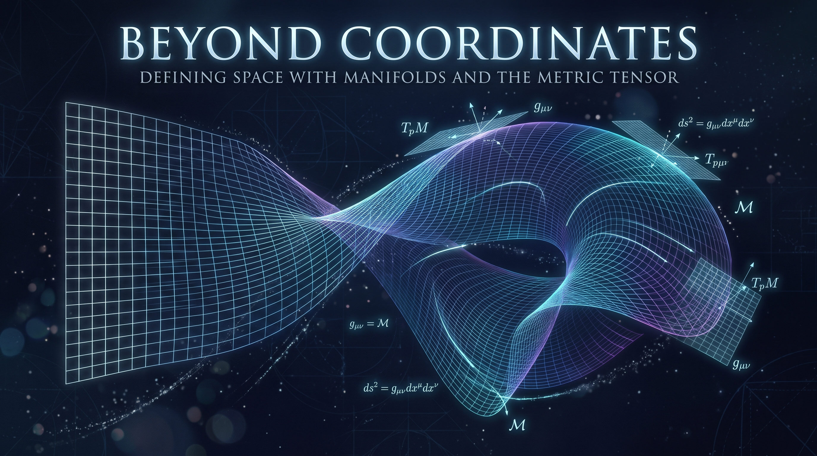
At school, space is a grid of axes, and Pythagoras gives us distance. But the Earth resists a single, distortion-free flat map. Gauss helped establish a deeper point: a surface’s curvature is intrinsic, and no choice of map can eliminate it.
Manifolds
The nineteenth-century answer, from Gauss and then Riemann in his famous 1854 lecture, was to stop demanding one map and use many.
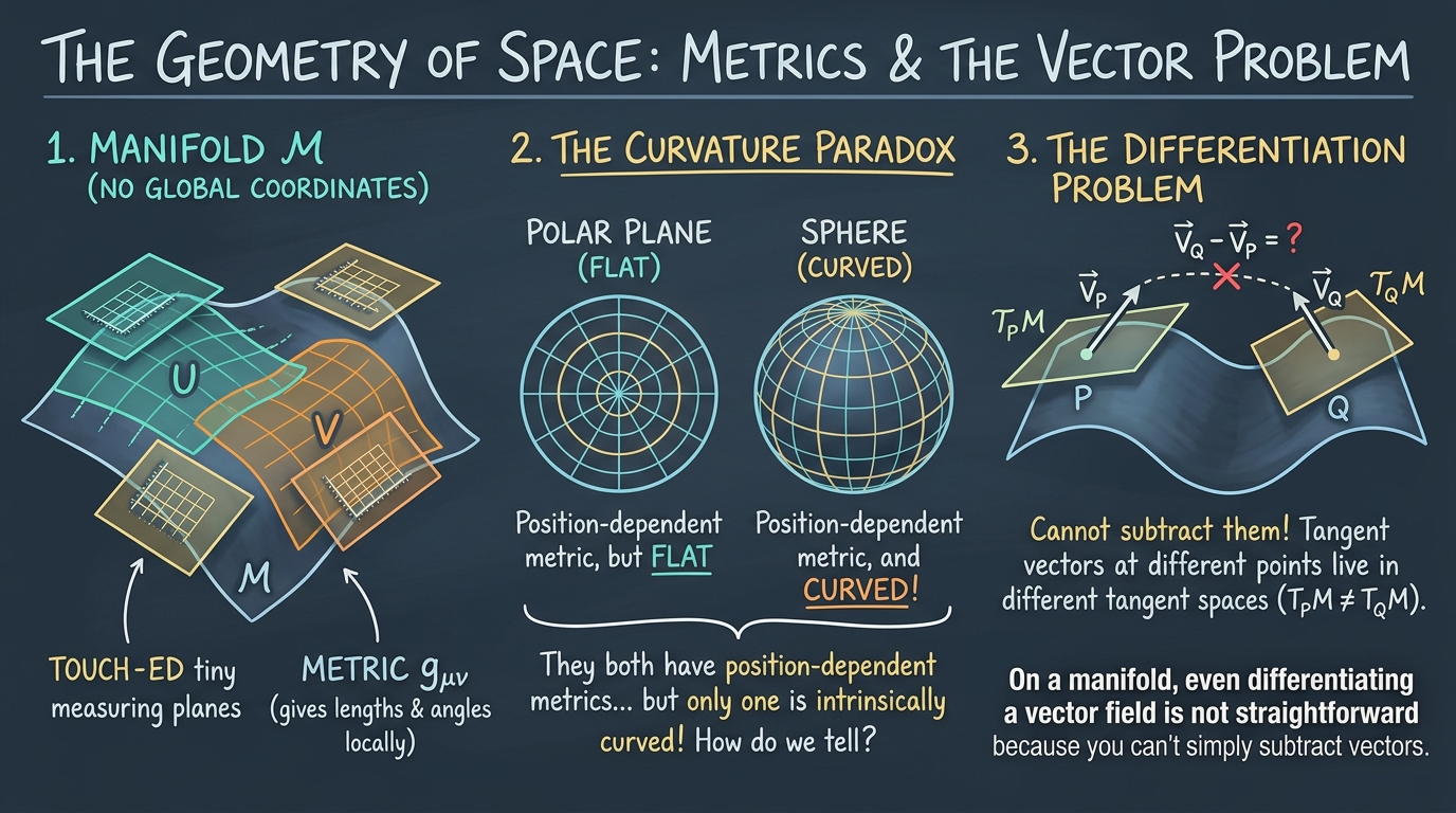
Standing in a field, the ground looks flat. In the same way, small regions of a curved space can be described with ordinary Euclidean coordinates. We call each local map a chart, and a collection of charts covering the whole space an atlas.
Where two charts overlap, one point gets two sets of coordinates, and the conversion between them must be infinitely differentiable. A space with such a compatible atlas is a smooth manifold, subject to a few technical conditions that rule out pathological examples.
The Metric Tensor
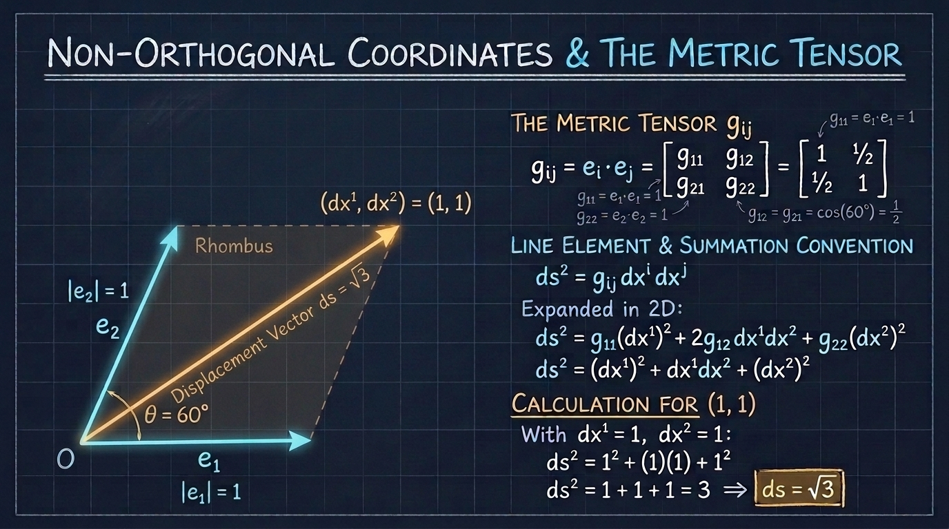
Imagine two axes meeting at sixty degrees, each with unit length. Because they aren’t perpendicular, the law of cosines adds a cross term to the squared distance.
We collect the coefficients into the metric tensor, written $g$ with two lower indices. The diagonal entries are one, and the off-diagonal entries are one half. With the summation convention, where repeated indices are added up, the whole rule fits in one line.
Try it on the displacement $(1, 1)$. The squared length is one plus one plus one, so the length is the square root of three.
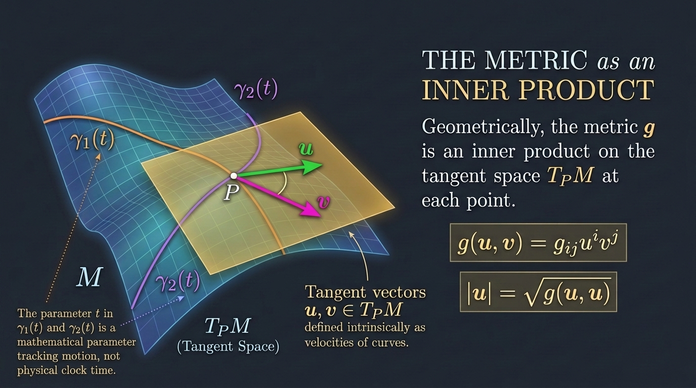
Geometrically, the metric is an inner product on the tangent space at each point. Tangent vectors don’t need a surrounding space; they can be defined intrinsically, as velocities of curves. We write $g(u, v)$ for the inner product of two tangent vectors $u$ and $v$, and in coordinates this is $g_{ij} u^i v^j$. From the inner product we get lengths and angles. For a Riemannian metric, any nonzero vector has positive length.
Varying Components Are Not Curvature
Changing coordinates changes the metric’s components, even in a flat space. Write the plane in polar coordinates and substitute, and you get the formula below. The $r^2$ term varies from place to place, yet the plane is perfectly flat.
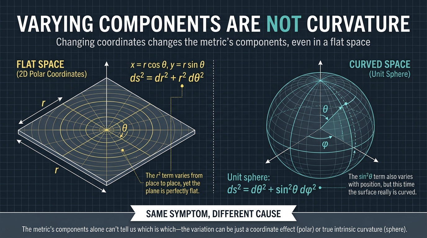
Now compare the unit sphere. Its metric components also vary with position, but this time the surface really is curved. Same symptom, different cause. The components alone can’t tell us which is which, and that is the question we will build toward over the next few episodes.
Raising and Lowering Indices
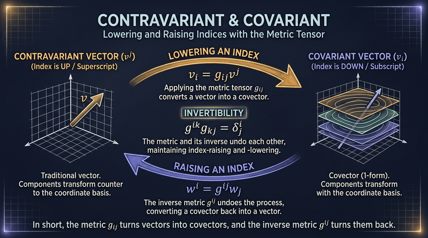
The metric also connects vectors to covectors. Applying the metric to vector components gives covector components, which is called lowering an index. Since the metric is invertible, its inverse undoes the process, called raising an index. In short, the metric turns vectors into covectors, and the inverse metric turns them back.
Contravariant and Covariant
Why do vector components use upper indices and covector components lower ones? And why are they called contravariant and covariant?
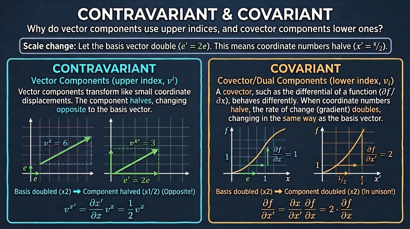
To see the difference, change the scale of a coordinate axis. Replace $x$ with $x' = x/2$. Equivalently, the basis vector doubles. The same physical position now gets a number half as large:
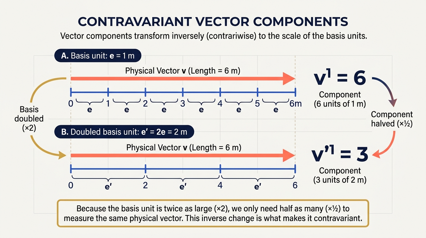
Contravariant. Vector components transform like small coordinate displacements, so the component also halves. It changes opposite to the basis vector — hence contra-variant.
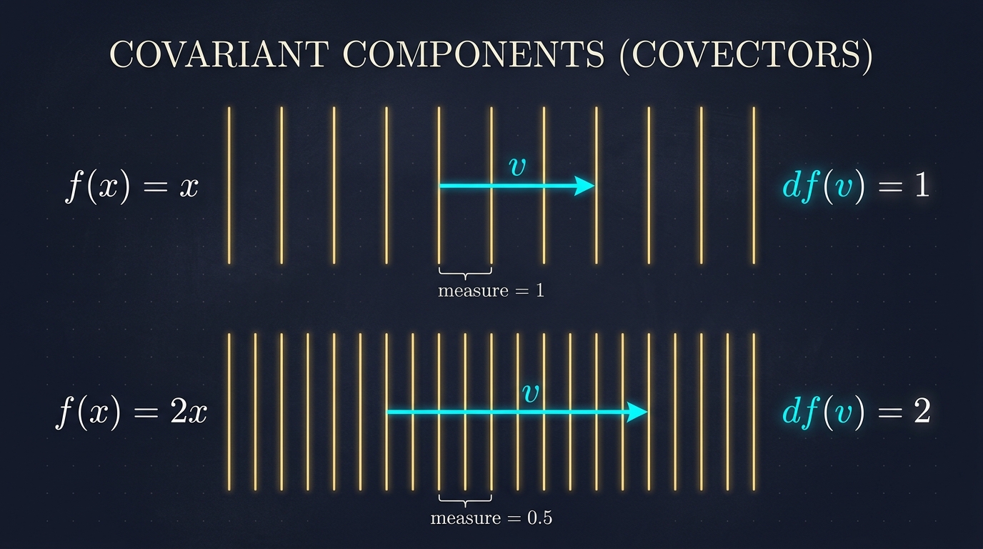
Covariant. A covector, such as the differential of a function $f$, behaves differently. Geometrically, it is a family of evenly spaced parallel lines, or planes: the level sets of $f$. Feed it a vector, and it returns the number of those lines the arrow crosses.
For $f(x)=x$, the level sets sit at $x=0,1,2,\dots$ (spacing $1$). For a unit vector $v$, $df(v)=1$ — one surface crossed per unit length. For $f(x)=2x$, the level sets sit at $x=0,0.5,1,1.5,\dots$ (spacing $0.5$). Now $df(v)=2$ — two surfaces per unit length. Tighter spacing ↔ larger $df$ ↔ steeper slope.
In components, this is the chain rule. The derivative with respect to the new coordinate picks up the opposite factor. When the coordinate numbers halve, the covector component doubles. It changes in the same way as the basis vector — hence co-variant:
Closing
Today we defined space without a single global coordinate system, then gave it lengths through the metric.
This is not just geometry for its own sake. In general relativity, spacetime itself is a manifold with a metric, and gravity is its geometry. We will come back to that at the end of the series.
But first, a problem. The polar plane and the sphere both have position-dependent metrics, and only one is curved. And on a manifold, even differentiating a vector field is not straightforward, because tangent vectors at different points live in different spaces, so we can’t simply subtract them.
Next time, we build the tool that fixes this: the connection. It tells us how to compare vectors at nearby points, and it is the first step toward measuring curvature.