The Threshold of Curvature — Differentiating in Curved Spaces: Connection and Parallel Transport
1. The Problem: Why the Partial Derivative Is Not a Tensor
In Foundations 6 we already met an uncomfortable fact: the partial derivative of a vector field $V^k$, namely $\partial_j V^k$, is not a tensor. Change coordinates and a “junk term” containing second derivatives pops out.
The reason is simple. Differentiating the vector field $V = V^i e_i$ produces two terms by the product rule:
The first term is the change of the components; the second is the change of the basis vectors. In Cartesian coordinates the $e_i$ are constant, so the second term vanishes. But in curvilinear coordinates and in curved spaces the basis vectors change from point to point. Differentiating only the components, while ignoring the change of the basis, yields noise that depends on the choice of coordinates.
A caution about the formula above: on a curved space, $\partial_j e_i$ is not yet well defined. The basis vector $e_i$ at one point and at a neighboring point live in different tangent spaces, so their difference has no meaning until we are told how to compare them. Supplying that missing rule is the job of a connection, introduced in the next section.
In Foundations 5 we learned that the Christoffel symbols $\Gamma^k{}_{ji}$ are precisely the device that records this change of basis:
Before we use them, we need to be clear about what they are coefficients of.
2. The Missing Ingredient: A Connection
The root of the difficulty is geometric. On a curved space, each point $p$ has its own tangent space $T_pM$. A vector $V(p)\in T_pM$ and a vector $V(q)\in T_qM$ belong to different vector spaces, so the difference quotient
has no meaning: you cannot subtract vectors from different spaces. In flat space we hide this problem because we can slide every arrow back to a common origin. On a curved space there is no canonical way to do that.
To differentiate, we must therefore add structure: a rule that tells us how to compare nearby tangent spaces. That rule is called a connection (the name reflects that it “connects” neighboring tangent spaces).
The first property says the derivative depends linearly on the direction. The second is the Leibniz (product) rule: differentiating $fV$ gives the change of the function times $V$, plus $f$ times the change of $V$.
These two rules are all we need to write $\nabla$ in coordinates. Expand $V = V^i e_i$ and $X = X^j e_j$. The Leibniz rule reduces everything to knowing how the basis vectors change, and that is recorded by a set of numbers:
The numbers $\Gamma^k{}_{ji}$ are the connection coefficients. In Foundations 5 we met them as the Christoffel symbols: the Christoffel symbols are the connection coefficients of one particular connection, the Levi-Civita connection.
The picture to keep: a connection is the rule for comparing vectors at neighboring points. The covariant derivative is the derivative that rule produces, and parallel transport is “keep the vector unchanged according to that rule.”
3. The Covariant Derivative: Differentiating the Basis Along with Everything Else
With the connection coefficients in hand, we can write the covariant derivative of a vector field in components:
Read it as: “differentiate $V$ in the $x^j$ direction, but add the part coming from the changing basis.”
To differentiate along an arbitrary direction $X = X^j e_j$ rather than a coordinate direction, contract with $X$:
This is the form used below, where $X$ will be the tangent vector $\dot\gamma$ of a curve.
How to read the symbols
These two symbols are read differently, and the difference matters for how you say the formulas aloud.
| Symbol | Spoken | Full phrase | What it does |
|---|---|---|---|
| $\partial_j$ | “partial j” | “partial with respect to $x^j$” | components only |
| $\nabla_j$ | “nabla j” | “covariant derivative in the $x^j$ direction” | components + basis change |
So the vector and covector formulas of this section read aloud as: “nabla j V k equals partial j V k plus Gamma k j i V i,” and “nabla j omega i equals partial j omega i minus Gamma k j i omega k.” The subscript $j$ is not summed over here — it labels which direction you differentiate in. Summation happens only on repeated upper–lower pairs inside the expression.
Why does this become a tensor? Apply the Leibniz rule to $V = V^i e_i$ and use the definition of the connection coefficients:
where in the first term we relabeled the dummy index $i \to k$. That is, $\nabla_j V^k$ are the components of the derivative of the whole vector field. Because the change of basis is already included, it transforms cleanly as a $(1,1)$ tensor under a change of coordinates.
For a covector (lower index) the sign flips:
The sign difference arises because upper and lower indices respond oppositely to a change of basis. It is the same contravariant/covariant symmetry we saw in Foundations 6. The minus sign is what keeps the pairing $\omega_i V^i$ obeying the ordinary product rule:
4. Parallel Transport: What It Means to Carry “the Same Vector” Along a Curve
Now we come to the geometrically most important concept.
In Euclidean space we can carry an arrow from one point to another “unchanged”: keep its direction and length, change only its base point. But in a curved space we must first define what “unchanged” means, because the tangent space at each point is a different space.
The definition is made with the covariant derivative. A vector field $V$ defined along a curve $\gamma(t)$ is parallel transported when
that is, when its covariant derivative in the direction of the curve’s tangent vector vanishes. In components:
This is a first-order linear ODE for $V^k$. Given an initial vector $V(0)$, the solution exists and is unique. Parallel transport therefore defines a linear isomorphism between the tangent spaces at different points.
In Euclidean space $\Gamma = 0$, so the equation reduces to $dV^k/dt = 0$: the components are constant. This matches exactly the intuition of carrying an arrow unchanged.
On a sphere, parallel transport is far more interesting. Carry a vector from the north pole down a meridian to the equator, then $90^\circ$ along the equator, then back up to the north pole. The vector returns pointing in a different direction than it started.
5. Geodesics: The Curve That Parallel-Transports Its Own Tangent
The most natural application of parallel transport is the geodesic. A geodesic is defined as a curve that parallel-transports its own tangent vector along itself:
In components this gives the geodesic equation:
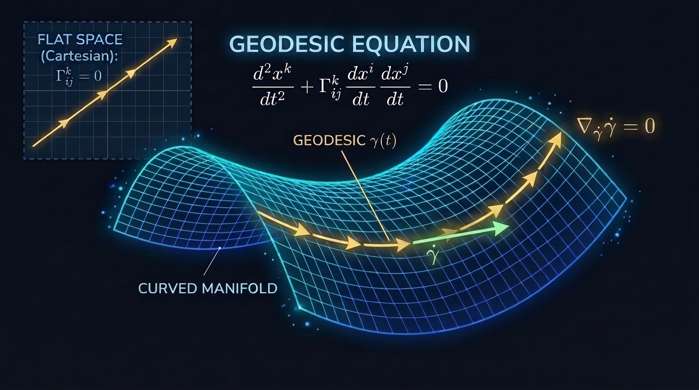
In Euclidean space, $\Gamma = 0$ gives $d^2x^k/dt^2 = 0$, which is uniform straight-line motion. In a curved space the geodesic is the generalization of that straight line. The worldline of a freely falling particle in a gravitational field obeys exactly this equation, and in Part 8 we will see how Einstein turns this fact into gravity itself.
6. Christoffel Symbols Are Not a Tensor — and That Is the Point
As emphasized in Foundations 6, $\Gamma^k{}_{ji}$ is not a tensor. Its transformation law carries a second-derivative term:
The second term is the “non-tensorial” part. But look at the definition of the covariant derivative: this junk term is engineered to cancel exactly against the junk term in $\partial_j V^k$. Precisely because the Christoffel symbols are not a tensor, they can combine with the non-tensorial partial derivative to produce something that is a tensor.
7. Looking Ahead
So far we have:
- seen why the partial derivative is not a tensor,
- built the covariant derivative by adding the Christoffel symbols,
- and used it to define parallel transport and geodesics.
The remaining question is this: if parallel transport depends on the path, what quantity measures the size of that dependence? How much a vector rotates when parallel transported around a closed loop — that rotation is curvature.