Covectors and Dual Space: What Is $dx^i$?
1. A Machine That Eats Vectors
In Foundations 3, we saw that a tangent vector is a directional-derivative operator. Now we turn the question around: what objects take a vector as input and return a number?
A covector at $p$ is a linear map $\alpha: T_pM \to \mathbb{R}$. Linear means that scaling a vector scales the output, and adding two vectors adds the outputs:
All covectors at $p$ form a vector space of their own, the dual space $T_p^*M$. It has the same dimension $n$ as $T_pM$.
In the plane, $dx$ is the covector that returns the horizontal component of a vector, and $dy$ the vertical one. For a vector with components $(a, b)$, $dx(v)=a$ and $dy(v)=b$. Any covector is a mix of these: $\alpha(v)=\alpha_1 a+\alpha_2 b$.
2. The Dual Basis
Choose coordinates, so that $\partial_1,\dots,\partial_n$ is a basis of $T_pM$. The dual basis $dx^1,\dots,dx^n$ is the set of covectors defined by:
Each $dx^i$ returns $1$ on its own basis vector and $0$ on all the others.
Any covector can be written in this basis, and its components are what it does to the basis vectors:
So the equation $\alpha = \alpha_i\,dx^i$ reads: “the covector $\alpha$ equals the number $\alpha_1$ times the covector $dx^1$, plus $\alpha_2$ times $dx^2$, plus …” It is a linear combination of covectors with scalar coefficients, which is again a covector.
Apply $\alpha$ to $v = v^j\partial_j$ and use linearity:
This is the pairing from Foundations 2: one lower index, one upper index, summed.
3. What Is $dx^i$, Really?
So far, we defined $dx^i$ by what it does. Here is what it is. For any smooth function $f$, its differential $df$ is the covector:
In words, $df$ feeds the vector to $f$ as a directional derivative. Apply this to the coordinate function $f = x^i$, and use $\partial_j(x^i)=\delta^i_j$ from Foundations 3:
So $dx^i$ really is the differential of the function $x^i$, and it extracts the $i$-th component of a vector. The two definitions agree. In general, $df$ expands in the dual basis with components $\partial_i f$:
You can check this by feeding it $\partial_j$: both sides give $\partial_j f$.
4. A Picture of a Covector
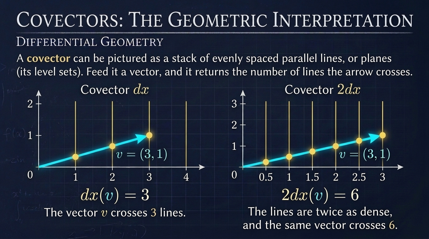
A covector can be pictured as a stack of evenly spaced parallel lines, or planes: its level sets. Feed it a vector, and it returns the number of lines the arrow crosses.
The covector $dx$ is the stack of vertical lines $x = 0, 1, 2, \dots$. The vector with components $(3, 1)$ crosses three of them, so $dx(v) = 3$. The covector $2\,dx$ has lines twice as dense, and the same vector crosses six.
5. Behavior Under Coordinate Changes
Change to new coordinates $\tilde{x}^i$. The chain rule gives:
The dual basis transforms by $A^{-1}$, opposite to the basis vectors $\partial_i$, which transform by $A$. The covector components must therefore transform by $A$, like the basis vectors:
Check that the pairing is invariant:
This is Foundations 1 with the roles swapped, and it matches the table in Foundations 2: lower index, transforms by $A$.
6. A Common Confusion
The symbol $dx^i$ is not an infinitesimal number, and it is not a vector either. It is a function that eats vectors.
There is a related trap. The differential $df$ is a covector, while the gradient $\nabla f$ from calculus is a vector. Turning one into the other needs the metric, with inverse metric $g^{ij}$:
In Cartesian coordinates, $g^{ij}=\delta^{ij}$, so the two look identical, which hides the distinction.
7. Where Does This Lead?
We now have both kinds of objects: vectors $v = v^i\partial_i$ and covectors $\alpha = \alpha_i\,dx^i$. But the basis $\partial_i$ and its dual $dx^i$ change from point to point, as we noticed at the end of Foundations 3. How they change is measured by the Christoffel symbols.