Convolution Explained: Why We Flip, Slide, Multiply, and Add
1. The mystery of convolution
Convolution has a bad reputation.
For many students, the first encounter goes something like this: you see a fearsome integral,
and wonder, “Wait. Why are we multiplying two functions? Why is one of them suddenly going backwards? And why are we integrating over a variable called tau?”
At that point, convolution can feel less like mathematics and more like a mathematical prank.
But here’s the surprising thing: the formula isn’t an arbitrary trick. It answers a very natural question.
Once you see the answer, convolution stops looking like something you have to memorize—and starts looking like something you could have discovered for yourself.
2. A system that remembers
Imagine striking a bell with a hammer.
The strike is almost instantaneous, but the sound continues long after the hammer makes contact. The bell rings, vibrates, and gradually falls silent.
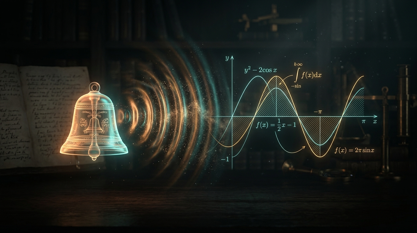
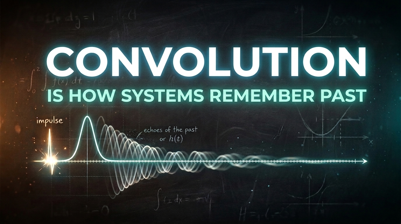
In mathematics and engineering, we describe the response to a single, idealized impulse with a function called the impulse response, written as $h(t)$.
Now imagine striking the bell several times, at different moments and with different strengths.
What will we hear?
The answer rests on a principle called superposition. For a linear system, the response to a combination of inputs is the combination of the individual responses.
And for a time-invariant system, shifting an input in time shifts its response by the same amount.
So we can think of a complicated input as a collection of tiny impulses. Each impulse produces its own copy of the bell’s ringing, starting at the moment of that impulse and scaled by its strength.
To find the total sound at time $t$, we add together all the contributions.
For a continuous input, those contributions become infinitesimally small, and adding them all becomes integration.
This gives us the convolution integral:
Here, $x$ is the input, $h$ is the impulse response, and $y$ is the output.
Now look at that expression $h(t-\tau)$.
Why the minus sign?
Because an impulse that occurred at time $\tau$ has been ringing for $t$ minus $\tau$ seconds by the time we observe the output at time $t$.
We’re measuring elapsed time, not the clock time when the impulse occurred.
The minus sign isn’t an arbitrary trick. It keeps track of how long each contribution has been developing.
And that gives us the physical meaning of convolution: adding up the shifted responses to all the pieces of an input.
3. Flip, slide, multiply, and add
Let’s make this idea concrete with a discrete example.
Suppose our input is
and our filter is
We want to calculate their convolution:
Rather than memorize the formula, let’s build the answer one output at a time.
Step one: Flip. Reverse the filter $[4, 5]$ to get $[5, 4]$.
Step two: Slide. Move the reversed filter across the input, one position at a time. Each position corresponds to a different output index $n$.
Step three: Multiply and add. Multiply the values that overlap, then add those products together.
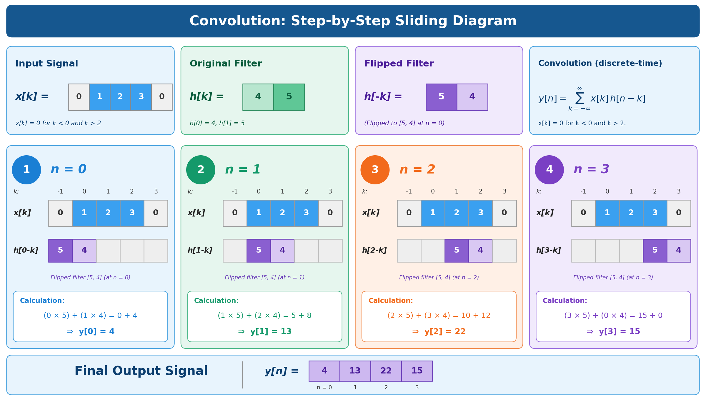
Let’s watch what happens.
At $n$ equals zero, only the first input value contributes. One times four gives four.
So $y[0]$ equals four.
At $n$ equals one, the contributions are one times five and two times four. Five plus eight gives thirteen.
So $y[1]$ equals thirteen.
At $n$ equals two, we multiply two by five and three by four. Ten plus twelve gives twenty-two.
So $y[2]$ equals twenty-two.
Finally, at $n$ equals three, only the last input value contributes. Three times five gives fifteen.
So $y[3]$ equals fifteen.
Our final output is
Notice that the output has four values. For two finite sequences of lengths three and two, the full linear convolution has length three plus two minus one, which is four.
And there’s another important detail: the indices of every contributing pair add up to $n$. That’s exactly what the expression $n-k$ tells us.
4. Two ways to see the same operation
Let’s return to the bell.
Our input $[1, 2, 3]$ represents three impulses: one at time zero, two at time one, and three at time two.
Each impulse produces a scaled copy of the response $[4, 5]$.
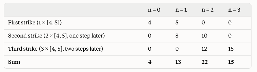
The first impulse contributes
The second contributes
because it occurs one time step later and has twice the strength.
The third contributes
because it occurs two steps later and has three times the strength.
Add the three responses, and we get
exactly the same result as our sliding calculation.
These are two views of the same process.
The sliding view asks: at a particular output position, which input and filter values overlap?
The bell view asks: how does each input value contribute to the entire output?
The sliding view looks at the output, one position at a time. The bell view looks at each input and follows its contribution through time.
Together, they reveal what convolution really does: it combines shifted copies of a response, weighted by the input.
5. Why the reversal matters
You might still wonder: what if we slide the filter without flipping it?
For our example, that produces
instead of
That’s a different operation, commonly called cross-correlation.
Both convolution and correlation are useful, but they aren’t generally the same when the filter is asymmetric.
In convolution, the reversal follows from the way we calculate the elapsed time between an input and an output. It isn’t decoration.
And once we understand that, the formula becomes much less mysterious.
6. The surprising payoff: convolution becomes multiplication
Now comes one of the most remarkable facts in mathematics.
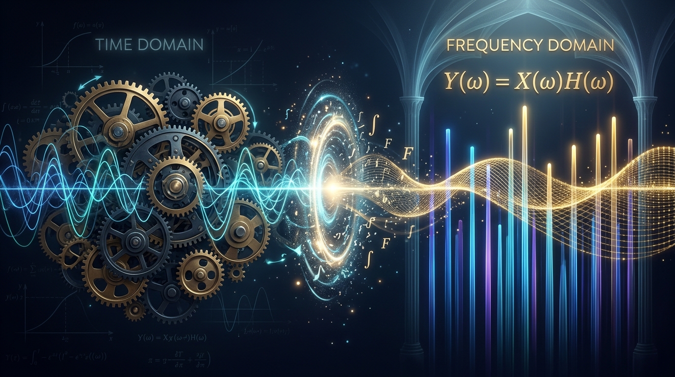
In the time domain, convolution requires us to slide, multiply, and add.
But take the Fourier transform, and convolution becomes ordinary multiplication:
Here, $X$, $H$, and $Y$ are the Fourier transforms of the input, impulse response, and output.
Why is that useful?
Because we can understand a system frequency by frequency. A filter might weaken high frequencies, preserve low frequencies, or amplify a particular range.
This is one of the ideas behind audio equalizers, image blurring, and many other signal-processing techniques.
The Fourier transform also helps us calculate large convolutions efficiently using the Fast Fourier Transform, or FFT.
Direct convolution can require many multiplications for long sequences. With suitable FFT-based methods, we can often calculate the same result much faster.
An operation that is complicated in one domain becomes simpler in another.
7. One more connection: polynomial multiplication
There’s another beautiful connection hiding in our original example.
Convolution is exactly the rule used to multiply polynomials by combining their coefficients.
Take these two polynomials:
and
Multiply them:
Look at the coefficients: four, thirteen, twenty-two, and fifteen.
They’re precisely the values of our convolution.
This isn’t a coincidence. When we multiply polynomials, every coefficient in the result is the sum of products of coefficients whose powers add up to the same exponent.
That’s the same rule as discrete convolution.
So the operation we’ve been studying connects signal processing, polynomial multiplication, and frequency analysis.
Conclusion: convolution is how a system remembers
Let’s return to our original question.
If we know how a linear, time-invariant system responds to a single impulse, how can we predict its response to an arbitrary input?
Break the input into impulses. Shift the system’s response to match each one. Scale each response by the strength of its input, then add them all together.
That’s convolution.
The reversal, the sliding, and the integral aren’t arbitrary tricks. They’re the mathematical bookkeeping required to assemble a system’s complete response from its individual reactions.
And in the frequency domain, that same operation becomes multiplication.
So convolution is more than a formula for combining two functions.
Once you see that, the formula stops being something you have to memorize—and becomes something you can understand for yourself.